The Simple Data Analysis library

In this lesson, we will learn how to use the open-source library I created: simple-data-analysis. We will analyze historical daily average temperature data in three Canadian cities as an example. Our goal will be to answer this question:

How fast have temperatures risen in the past decades?

To do that, we will calculate the average temperature per 30-year period and check for trends.

If you have a minute, please add a ⭐ to the library’s GitHub repository. It’s always nice to know your open-source work is appreciated. 😊

Note that I expect you to have at least completed the First steps 🧑‍🎓 and Pushing further 🚀 sections.

Want to know when new lessons are available? Subscribe to the newsletter ✉️ and give a ⭐ to the GitHub repository to keep me motivated! Click here to get in touch.

Setup

The library is published on JSR, and you can install it by running deno add @nshiab/simple-data-analysis.

But there’s a better way. 😏

Create a new folder on your computer and run this instead: deno -A jsr:@nshiab/setup-sda

This tells Deno to run another library called setup-sda, which I also created to easily install and set up everything needed when starting a new data analysis.

After running the command, your terminal will display a description of the created files and installed libraries.

A screenshot showing VS Code after running setup-sda.

💡

For SDA to work properly, it’s best to have at least version 2.1.9 of Deno. To check your version, you can run deno --version in your terminal. To upgrade it, simply run deno upgrade.

Files created

deno.json: If you click on it, you’ll see two tasks. We will use sda to watch, check, and run sda/main.ts. You can also see three libraries listed. More about them below.
.gitignore: An important file when using git to save our code. Don’t worry about it for now; there will be a full lesson about it.
sda/main.ts: The main file of our script. We will write our code here.
sda/helpers: An empty folder for now, but you can use it to store your functions.
sda/data: An empty folder for now, but this is where we will store our data for analysis.
sda/output: An empty folder for now. This is where we will write our results into files.
README.md: A text file containing some information about the project. You can modify it as you wish.

Libraries installed

simple-data-analysis: The library we will use to process the data.
journalism: Another library I created. It contains useful functions for various tasks, like formatting dates or pushing data to Google Sheets.
@observablehq/plot: A library created by Mike Bostock (creator of d3.js) that we will use to create charts and maps.

Now that you know what’s in your folder, let’s start working. Run the suggested task to run and watch our code: deno task sda

Creating a table

Let me explain the current code in ./sda/main.ts.

When you use SDA, you create an in-memory database. This is what happens on line 3 with const sdb = new SimpleDB(). When we are done with our computations, we close the database on line 7 with await sdb.done().

main.ts

import { SimpleDB } from "@nshiab/simple-data-analysis";
 
const sdb = new SimpleDB();
 
// Do your magic here!
 
await sdb.done();

As in a regular database, with SimpleDB, data is stored in tables. If you are more familiar with Excel or Google Sheets, tables can be understood as tabs.

Let’s create one to store daily temperatures.

To create a table, you can use the .newTable() method. You can give it a name (though it’s optional) and store the table in a variable. Usually, I name the variable and the table the same thing.

main.ts

import { SimpleDB } from "@nshiab/simple-data-analysis";
 
const sdb = new SimpleDB();
 
const temperatures = sdb.newTable("temperatures");
 
await sdb.done();

Now that we have a table, we can use the table’s methods! On another line, type the variable temperature (which now refers to the table) and add a . immediately after it to see all the available methods. You can use your up and down keyboard arrows to check their documentation and examples. There’s a lot!

All the methods documented with examples are also available on JSR.

In the screenshot below, I stopped on loadData, which is the method we are going to use in a minute.

A screenshot showing VS Code documentation for loadData.

Loading data

I uploaded historical daily temperatures for three Canadian cities to GitHub. It’s a CSV file that you can see here. It comes from the Adjusted and Homogenized Canadian Climate Data from Environment Canada.

Let’s use the loadData method to retrieve it. Note that the method can fetch remote files as well as read local files. It can parse CSV, JSON, Excel, and Parquet files. Quite handy!

It would be nice to see the data once loaded. We can do that by calling the logTable method.

All table methods are async, so we need to specify await in front of them.

main.ts

import { SimpleDB } from "@nshiab/simple-data-analysis";
 
const sdb = new SimpleDB();
 
const temperatures = sdb.newTable("temperatures");
 
await temperatures.loadData(
  "https://raw.githubusercontent.com/nshiab/simple-data-analysis/refs/heads/main/test/data/files/dailyTemperatures.csv",
);
 
await temperatures.logTable();
 
await sdb.done();

And here’s the result! We can see the CSV data has been ingested into the table temperature, which now has three columns and 131k rows.

A screenshot showing temperature data logged in the terminal.

Joining data

It would be better to replace the IDs with the city names. The IDs and the city names are in another file that I uploaded on GitHub too.

Let’s fetch it too.

main.ts

import { SimpleDB } from "@nshiab/simple-data-analysis";
 
const sdb = new SimpleDB();
 
const temperatures = sdb.newTable("temperatures");
await temperatures.loadData(
  "https://raw.githubusercontent.com/nshiab/simple-data-analysis/refs/heads/main/test/data/files/dailyTemperatures.csv",
);
await temperatures.logTable();
 
const cities = sdb.newTable("cities");
await cities.loadData(
  "https://raw.githubusercontent.com/nshiab/simple-data-analysis/refs/heads/main/test/data/files/cities.csv",
);
await cities.logTable();
 
await sdb.done();

A screenshot showing the cities names in the terminal.

Now, we want to bring the city names into the temperature table. To do that, we can use the .join() method.

By default, this method looks for a common column in two tables and matches rows based on the values in this column.

So, when we write await temperature.join(cities), we ask SDA to find a common column (which is id) in temperature and cities and to add the cities values with the same id to the corresponding temperature rows.

Note that I commented out the previous logTable calls on lines 9 and 15 to avoid clogging the terminal.

main.ts

import { SimpleDB } from "@nshiab/simple-data-analysis";
 
const sdb = new SimpleDB();
 
const temperatures = sdb.newTable("temperatures");
await temperatures.loadData(
  "https://raw.githubusercontent.com/nshiab/simple-data-analysis/refs/heads/main/test/data/files/dailyTemperatures.csv",
);
// await temperatures.logTable();
 
const cities = sdb.newTable("cities");
await cities.loadData(
  "https://raw.githubusercontent.com/nshiab/simple-data-analysis/refs/heads/main/test/data/files/cities.csv",
);
// await cities.logTable();
 
await temperatures.join(cities);
await temperatures.logTable();
 
await sdb.done();

And now we have the city names in the temperature table!

A screenshot showing the city names in the temperature table.

Caching

Currently, every time we save main.ts, the two CSV files are being refetched. This is slow and unnecessary since the data doesn’t change.

Let’s cache everything we’ve done so far with the .cache() method.

You can wrap code inside an async function and pass it to .cache(). The first time this code runs, SDA will fetch the data and perform the necessary computations before writing the results into the .sda-cache folder.

Here, I set the cacheVerbose option to true when instantiating SimpleDB to log cache-related information in the terminal.

main.ts

import { SimpleDB } from "@nshiab/simple-data-analysis";
 
const sdb = new SimpleDB({ cacheVerbose: true });
 
const temperatures = sdb.newTable("temperatures");
 
await temperatures.cache(async () => {
  await temperatures.loadData(
    "https://raw.githubusercontent.com/nshiab/simple-data-analysis/refs/heads/main/test/data/files/dailyTemperatures.csv",
  );
  // await temperatures.logTable();
 
  const cities = sdb.newTable("cities");
  await cities.loadData(
    "https://raw.githubusercontent.com/nshiab/simple-data-analysis/refs/heads/main/test/data/files/cities.csv",
  );
  // await cities.logTable();
 
  await temperatures.join(cities);
});
 
await temperatures.logTable();
 
await sdb.done();

Here’s the result on the first run.

As indicated in the terminal, SDA didn’t find anything in cache for the code on lines 8 to 19, so it ran everything, and it took 1 sec, 441 ms with my internet connection and computer. .sda-cache has been created, and data is now cached in it.

A screenshot showing data being cached.

When I save main.ts again (CMD + S on Mac and CTRL + S on PC), it’s different.

SDA checked if the code between lines 8 and 19 had been modified. Since it’s exactly the same, it just loads the results of the previous run, which are stored in .sda-cache.

Instead of 1 sec, 441 ms, running the script took only… 32 ms! That’s 45 times faster! 😱

Here, most of the time saved is from fetching the data. But as we will see in other lessons, you can also cache the results of heavy computations that take a long time to run, which can significantly improve your productivity.

A screenshot showing data being retrieved from the cache.

💡

When using the .cache() method, it’s very important to call await sdb.done() at the end of your script. Among other things, this method removes unused cached data on each run. Without it, the cache could become very big. And if you want to manually clean your cache, just run deno task clean.

Exploring the data

To explore the data, we can use the .summarize() method. It aggregates the data in the table.

Let’s start with time. We specify the categories as the values in the city column to see the details for each city.

main.ts

import { SimpleDB } from "@nshiab/simple-data-analysis";
 
const sdb = new SimpleDB({ cacheVerbose: true });
 
const temperatures = sdb.newTable("temperatures");
 
await temperatures.cache(async () => {
  await temperatures.loadData(
    "https://raw.githubusercontent.com/nshiab/simple-data-analysis/refs/heads/main/test/data/files/dailyTemperatures.csv",
  );
  // await temperatures.logTable();
 
  const cities = sdb.newTable("cities");
  await cities.loadData(
    "https://raw.githubusercontent.com/nshiab/simple-data-analysis/refs/heads/main/test/data/files/cities.csv",
  );
  // await cities.logTable();
 
  await temperatures.join(cities);
});
 
await temperatures.summarize({
  values: "time",
  categories: "city"
});
await temperatures.logTable();
 
await sdb.done();

The min and max values show that we have over a hundred years’ worth of daily temperatures for our three cities. This is pretty good for checking trends!

But there is a problem… The count column has different values for each city. In theory, we should have around 44,195 days in 121 years. We see fewer than that here, which means we will have to deal with missing data…

A screenshot showing the time values aggregated.

💡

If the table layout is displayed weirdly in your terminal, it’s because the width of the table is bigger than the width of your terminal. Right-click on the terminal and look for Toggle size with content width. There is also a handy shortcut that I use all the time to do that: OPTION + Z on Mac and ALT + Z on PC.

Let’s now check what we have in t, which stands for temperature. Just replace "time" with "t" on line 23.

Hmm… Not only do we have missing rows in our data, as we saw just above, but we also have some rows with null values.

A screenshot showing the temperature values aggregated.

Let’s take care of this right away by using the .removeMissing() method. It removes any rows with a null value. You can also specify specific columns if needed, but it’s not necessary here.

Let’s put that in the cache while we’re at it.

main.ts

import { SimpleDB } from "@nshiab/simple-data-analysis";
 
const sdb = new SimpleDB({ cacheVerbose: true });
 
const temperatures = sdb.newTable("temperatures");
 
await temperatures.cache(async () => {
  await temperatures.loadData(
    "https://raw.githubusercontent.com/nshiab/simple-data-analysis/refs/heads/main/test/data/files/dailyTemperatures.csv",
  );
  // await temperatures.logTable();
 
  const cities = sdb.newTable("cities");
  await cities.loadData(
    "https://raw.githubusercontent.com/nshiab/simple-data-analysis/refs/heads/main/test/data/files/cities.csv",
  );
  // await cities.logTable();
 
  await temperatures.join(cities);
 
  await temperatures.removeMissing();
});
 
await temperatures.summarize({
  values: "time",
  categories: "city",
});
await temperatures.logTable();
 
await sdb.done();

Here we go! No more null temperatures.

Since we changed the code in the .cache() method, you’ll notice that the message in the terminal indicates that the code is being run again. Pretty clever, huh? 😉

A screenshot showing the removeMissing method.

Binning the years

One of my go-to resources when I want to analyze climate data is climatedata.ca. They have a great section about why you should use 30-year averages when looking for climate trends.

So this is what we are going to do here!

First, let’s add a new column with the time year. The .addColumn() method needs three arguments:

The name of the new column. Here, it’s year.
The type of the data in the column. Here, it’s number.
The definition of the data in the column. This is an SQL expression (more about it below). We want to extract the year from time.

main.ts

import { SimpleDB } from "@nshiab/simple-data-analysis";
 
const sdb = new SimpleDB({ cacheVerbose: true });
 
const temperatures = sdb.newTable("temperatures");
 
await temperatures.cache(async () => {
  await temperatures.loadData(
    "https://raw.githubusercontent.com/nshiab/simple-data-analysis/refs/heads/main/test/data/files/dailyTemperatures.csv",
  );
  // await temperatures.logTable();
 
  const cities = sdb.newTable("cities");
  await cities.loadData(
    "https://raw.githubusercontent.com/nshiab/simple-data-analysis/refs/heads/main/test/data/files/cities.csv",
  );
  // await cities.logTable();
 
  await temperatures.join(cities);
 
  await temperatures.removeMissing();
});
 
await temperatures.addColumn("year", "number", `YEAR(time)`);
await temperatures.logTable();
 
await sdb.done();

💡

YEAR(time) is a SQL expression. The Structured Query Language is a very common language when working with databases. Under the hood, SDA works in SQL. But don’t worry, you don’t have to be an expert in SQL to use SDA. When you need SQL, it will stay very basic, like in the example above, and we will learn the basics as we work on lessons and projects.

A screenshot showing the addColumn method.

Now, we can bin the years with the .bins() method. As you may start to understand, there is a SDA method to do pretty much anything you need when analyzing data. 😎

The method needs three arguments:

The column storing the values
The interval for the bins
The name of the new column storing the bins

Just to check if everything was done as expected, we can log the result of await temperature.getUniques("bin"), which will return all the unique values in the new column bin.

main.ts

import { SimpleDB } from "@nshiab/simple-data-analysis";
 
const sdb = new SimpleDB({ cacheVerbose: true });
 
const temperatures = sdb.newTable("temperatures");
 
await temperatures.cache(async () => {
  await temperatures.loadData(
    "https://raw.githubusercontent.com/nshiab/simple-data-analysis/refs/heads/main/test/data/files/dailyTemperatures.csv",
  );
  // await temperatures.logTable();
 
  const cities = sdb.newTable("cities");
  await cities.loadData(
    "https://raw.githubusercontent.com/nshiab/simple-data-analysis/refs/heads/main/test/data/files/cities.csv",
  );
  // await cities.logTable();
 
  await temperatures.join(cities);
 
  await temperatures.removeMissing();
});
 
await temperatures.addColumn("year", "number", `YEAR(time)`);
await temperatures.bins("year", 30, "bin");
await temperatures.logTable();
 
console.log(await temperatures.getUniques("bin"));
 
await sdb.done();

This is looking great!

A screenshot showing the bins and getUniques method.

Summarizing and filtering the data

Now that we have our daily temperatures binned properly, we can easily compute the average temperature per 30-year period for each city.

Let’s use our .summarize() method again. But this time, we will use more options:

The values are still our temperatures in the t column.
There are now two categories. We want to keep the cities and the bins!
We want the mean and a count of the values for each city and each bin.
We round the values to two decimals.

Also, the table now has 15 rows, but .logTable() just shows the first 10. So we ask it to log 15 to have a better look at the result.

main.ts

import { SimpleDB } from "@nshiab/simple-data-analysis";
 
const sdb = new SimpleDB({ cacheVerbose: true });
 
const temperatures = sdb.newTable("temperatures");
 
await temperatures.cache(async () => {
  await temperatures.loadData(
    "https://raw.githubusercontent.com/nshiab/simple-data-analysis/refs/heads/main/test/data/files/dailyTemperatures.csv",
  );
  // await temperatures.logTable();
 
  const cities = sdb.newTable("cities");
  await cities.loadData(
    "https://raw.githubusercontent.com/nshiab/simple-data-analysis/refs/heads/main/test/data/files/cities.csv",
  );
  // await cities.logTable();
 
  await temperatures.join(cities);
 
  await temperatures.removeMissing();
});
 
await temperatures.addColumn("year", "number", `YEAR(time)`);
await temperatures.bins("year", 30, "bin");
await temperatures.summarize({
  values: "t",
  categories: ["city", "bin"],
  summaries: ["mean", "count"],
  decimals: 2,
});
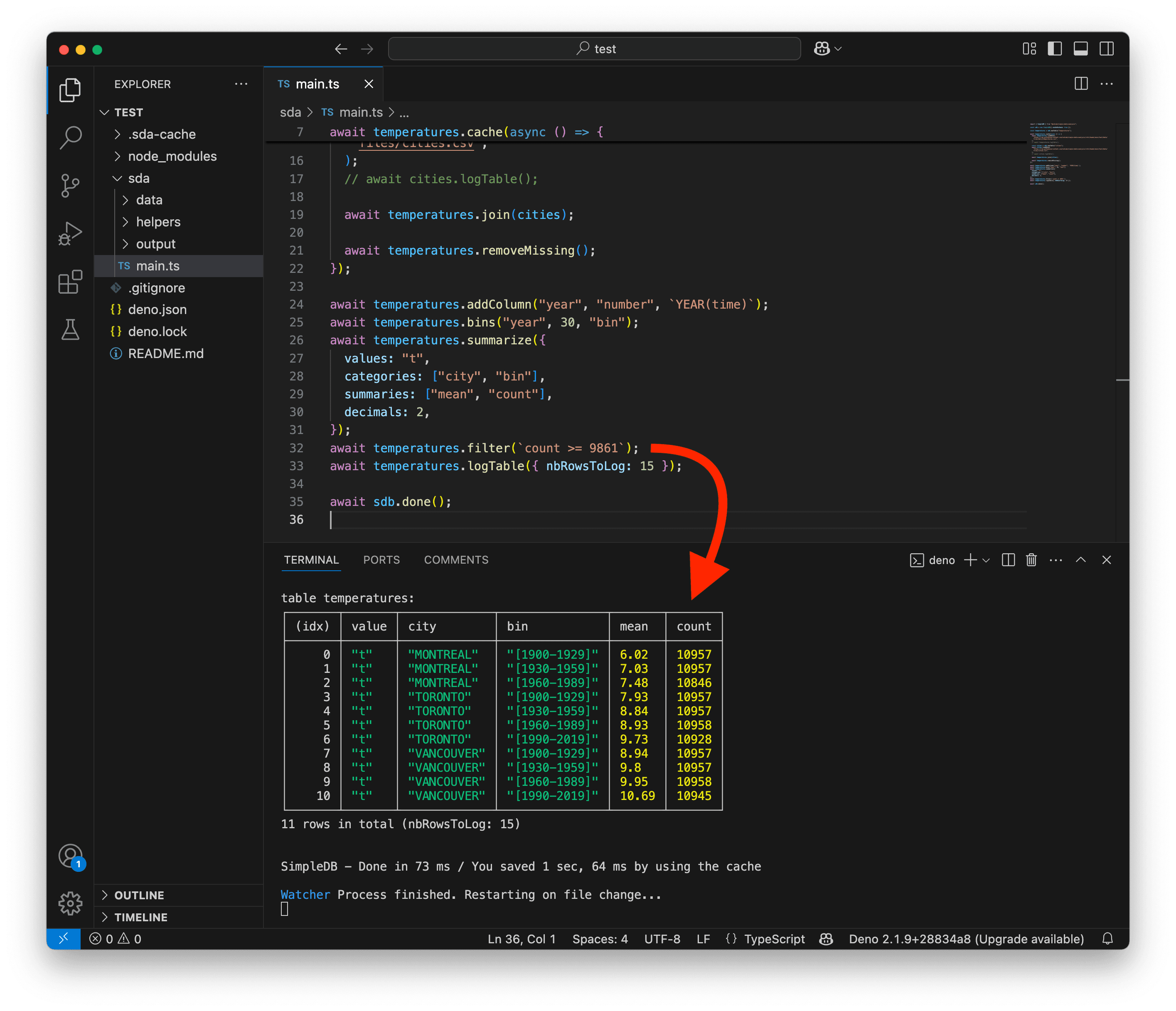
await temperatures.logTable({ nbRowsToLog: 15 });
 
await sdb.done();

This is looking very good. Thanks to the count, we can clearly see where data is missing.

Of course, the [2020-2049] bins are incomplete, but so is the [1990-2019] bin for MONTREAL. In theory, the 30-year bins should have around 10,957 days.

A screenshot showing the summary method.

We could filter out bins that have less than 90% of the expected number of days. So our threshold would be 9,861 days.

To do that, let’s use the .filter() method, which takes an SQL expression as a condition. As you can see below, it’s pretty simple.

main.ts

import { SimpleDB } from "@nshiab/simple-data-analysis";
 
const sdb = new SimpleDB({ cacheVerbose: true });
 
const temperatures = sdb.newTable("temperatures");
 
await temperatures.cache(async () => {
  await temperatures.loadData(
    "https://raw.githubusercontent.com/nshiab/simple-data-analysis/refs/heads/main/test/data/files/dailyTemperatures.csv",
  );
  // await temperatures.logTable();
 
  const cities = sdb.newTable("cities");
  await cities.loadData(
    "https://raw.githubusercontent.com/nshiab/simple-data-analysis/refs/heads/main/test/data/files/cities.csv",
  );
  // await cities.logTable();
 
  await temperatures.join(cities);
 
  await temperatures.removeMissing();
});
 
await temperatures.addColumn("year", "number", `YEAR(time)`);
await temperatures.bins("year", 30, "bin");
await temperatures.summarize({
  values: "t",
  categories: ["city", "bin"],
  summaries: ["mean", "count"],
  decimals: 2,
});
await temperatures.filter(`count >= 9861`);
await temperatures.logTable({ nbRowsToLog: 15 });
 
await sdb.done();

💡

You don’t have to use backticks for SQL expressions, like I wrote on lines 24 and 32. The methods just expect strings. Using backticks is just a habit I took because template literals are useful for injecting variables into strings, and it’s something we will often do with SQL expressions, as we will see in later lessons and projects.

We are now left with 11 rows.

A screenshot showing the filter method.

Trends

Reformatting

Whether we want to visualize the data or compute statistical indicators to check for trends, we have a problem: our bins are text. It would be much easier to have them as numbers.

This is what the code below does:

On line 33, we use the .splitExtract() method to split the bins on the - character, then pick the first part (index 0) and put it in a new column startYear.
On line 34, we trim the leftover [.
Finally, on line 35, we convert the values in the column startYear to number.

By the way, you can always hover over the methods to see their documentation and examples. I took the time to document each one of them. 🫡

main.ts

import { SimpleDB } from "@nshiab/simple-data-analysis";
 
const sdb = new SimpleDB({ cacheVerbose: true });
 
const temperatures = sdb.newTable("temperatures");
 
await temperatures.cache(async () => {
  await temperatures.loadData(
    "https://raw.githubusercontent.com/nshiab/simple-data-analysis/refs/heads/main/test/data/files/dailyTemperatures.csv",
  );
  // await temperatures.logTable();
 
  const cities = sdb.newTable("cities");
  await cities.loadData(
    "https://raw.githubusercontent.com/nshiab/simple-data-analysis/refs/heads/main/test/data/files/cities.csv",
  );
  // await cities.logTable();
 
  await temperatures.join(cities);
 
  await temperatures.removeMissing();
});
 
await temperatures.addColumn("year", "number", `YEAR(time)`);
await temperatures.bins("year", 30, "bin");
await temperatures.summarize({
  values: "t",
  categories: ["city", "bin"],
  summaries: ["mean", "count"],
  decimals: 2,
});
await temperatures.filter(`count >= 9861`);
await temperatures.splitExtract("bin", "-", 0, "startYear");
await temperatures.trim("startYear", { character: "[" });
await temperatures.convert({ startYear: "number" });
await temperatures.logTable({ nbRowsToLog: 15 });
 
await sdb.done();

A screenshot showing how to clean strings.

Visualization in the terminal

We can now easily visualize our data!

With SDA, you can create basic charts in your terminal. Here, we use .logDotChart(), and we can clearly see how temperatures have increased over the previous century.

main.ts

import { SimpleDB } from "@nshiab/simple-data-analysis";
 
const sdb = new SimpleDB({ cacheVerbose: true });
 
const temperatures = sdb.newTable("temperatures");
 
await temperatures.cache(async () => {
  await temperatures.loadData(
    "https://raw.githubusercontent.com/nshiab/simple-data-analysis/refs/heads/main/test/data/files/dailyTemperatures.csv",
  );
  // await temperatures.logTable();
 
  const cities = sdb.newTable("cities");
  await cities.loadData(
    "https://raw.githubusercontent.com/nshiab/simple-data-analysis/refs/heads/main/test/data/files/cities.csv",
  );
  // await cities.logTable();
 
  await temperatures.join(cities);
 
  await temperatures.removeMissing();
});
 
await temperatures.addColumn("year", "number", `YEAR(time)`);
await temperatures.bins("year", 30, "bin");
await temperatures.summarize({
  values: "t",
  categories: ["city", "bin"],
  summaries: ["mean", "count"],
  decimals: 2,
});
await temperatures.filter(`count >= 9861`);
await temperatures.splitExtract("bin", "-", 0, "startYear");
await temperatures.trim("startYear", { character: "[" });
await temperatures.convert({ startYear: "number" });
await temperatures.logTable({ nbRowsToLog: 15 });
 
await temperatures.logDotChart("startYear", "mean", { smallMultiples: "city" });
 
await sdb.done();

A screenshot showing how to log charts in the terminal.

Visualization with Plot

Visualizations in the terminal are quite limited. If you want to create fancier charts, you can use Observable Plot, which was installed when setting up with setup-sda.

We will do a full lesson on Plot later. It might seem complicated right now, but once you get the basics, it’s an amazing data visualization library.

In the example below, we write a chart as a PNG file in our ./sda/output folder.

main.ts

import { SimpleDB } from "@nshiab/simple-data-analysis";
import { dot, line, plot } from "@observablehq/plot";
 
const sdb = new SimpleDB({ cacheVerbose: true });
 
const temperatures = sdb.newTable("temperatures");
 
await temperatures.cache(async () => {
  await temperatures.loadData(
    "https://raw.githubusercontent.com/nshiab/simple-data-analysis/refs/heads/main/test/data/files/dailyTemperatures.csv",
  );
  // await temperatures.logTable();
 
  const cities = sdb.newTable("cities");
  await cities.loadData(
    "https://raw.githubusercontent.com/nshiab/simple-data-analysis/refs/heads/main/test/data/files/cities.csv",
  );
  // await cities.logTable();
 
  await temperatures.join(cities);
 
  await temperatures.removeMissing();
});
 
await temperatures.addColumn("year", "number", `YEAR(time)`);
await temperatures.bins("year", 30, "bin");
await temperatures.summarize({
  values: "t",
  categories: ["city", "bin"],
  summaries: ["mean", "count"],
  decimals: 2,
});
await temperatures.filter(`count >= 9861`);
await temperatures.splitExtract("bin", "-", 0, "startYear");
await temperatures.trim("startYear", { character: "[" });
await temperatures.convert({ startYear: "number" });
await temperatures.logTable({ nbRowsToLog: 15 });
 
const chart = (data: unknown[]) =>
  plot({
    inset: 20,
    marginLeft: 50,
    marginBottom: 40,
    grid: true,
    y: { tickFormat: (d) => `${d}°C`, label: "Temperature", ticks: 5 },
    x: {
      tickFormat: (d) => `${d}-${d + 29}`,
      ticks: [1900, 1930, 1960, 1990],
      label: "Year",
    },
    color: { legend: true },
    marks: [
      line(data, {
        x: "startYear",
        y: "mean",
        stroke: "city",
        curve: "natural",
      }),
      dot(data, {
        x: "startYear",
        y: "mean",
        fill: "white",
        stroke: "city",
        strokeWidth: 2,
        r: 4,
      }),
    ],
  });
await temperatures.writeChart(
  chart,
  "./sda/output/temperatures.png",
);
 
await sdb.done();

A screenshot showing how to write charts with Plot.

💡

You can open all kinds of files with VS Code, including images. Since we are watching main.ts, every time we update the code creating the chart, temperatures.png gets rewritten and updated in its tab. Another trick: you can grab the temperatures.png tab and place it wherever you want, including on a second screen if you have one.

Correlations and linear regressions

Now, visualizations are great, but their interpretation can be quite subjective.

For trends, you can also rely on statistical indicators like correlations and linear regressions. If you want to know more about this, check out the lesson Math for journalists.

Let’s start with correlations. Note that I removed the code to generate the chart.

Like .summarize(), the .correlations method replaces the data in the table with the result of its computations.

main.ts

import { SimpleDB } from "@nshiab/simple-data-analysis";
 
const sdb = new SimpleDB({ cacheVerbose: true });
 
const temperatures = sdb.newTable("temperatures");
 
await temperatures.cache(async () => {
  await temperatures.loadData(
    "https://raw.githubusercontent.com/nshiab/simple-data-analysis/refs/heads/main/test/data/files/dailyTemperatures.csv",
  );
  // await temperatures.logTable();
 
  const cities = sdb.newTable("cities");
  await cities.loadData(
    "https://raw.githubusercontent.com/nshiab/simple-data-analysis/refs/heads/main/test/data/files/cities.csv",
  );
  // await cities.logTable();
 
  await temperatures.join(cities);
 
  await temperatures.removeMissing();
});
 
await temperatures.addColumn("year", "number", `YEAR(time)`);
await temperatures.bins("year", 30, "bin");
await temperatures.summarize({
  values: "t",
  categories: ["city", "bin"],
  summaries: ["mean", "count"],
  decimals: 2,
});
await temperatures.filter(`count >= 9861`);
await temperatures.splitExtract("bin", "-", 0, "startYear");
await temperatures.trim("startYear", { character: "[" });
await temperatures.convert({ startYear: "number" });
 
await temperatures.correlations({
  x: "startYear",
  y: "mean",
  categories: "city",
});
await temperatures.logTable({ nbRowsToLog: 15 });
 
await sdb.done();

As we can see, the correlations are close to 1, meaning there is a strong relationship between the years and the temperature. When one goes up, the other goes up too.

A screenshot showing how to compute correlations.

We can also compute linear regressions, which are more descriptive. Just replace the .correlations method with .linearRegressions on line 37 and add the option decimals: 2 to round the values on line 41.

Again, the r² is close to 1, meaning the two variables are related. The slope also tells us that the temperature increased by 0.02°C each year on average.

These three Canadian cities warmed up! 🌡️🌡️🌡️

A screenshot showing how to compute linear regressions.

Writing data

For the sake of the lesson, let’s write our results to a file. With the .writeData() method, you can save CSV, JSON, and Parquet files. If you are working with big files, you have options available to compress them.

main.ts

import { SimpleDB } from "@nshiab/simple-data-analysis";
 
const sdb = new SimpleDB({ cacheVerbose: true });
 
const temperatures = sdb.newTable("temperatures");
 
await temperatures.cache(async () => {
  await temperatures.loadData(
    "https://raw.githubusercontent.com/nshiab/simple-data-analysis/refs/heads/main/test/data/files/dailyTemperatures.csv",
  );
  // await temperatures.logTable();
 
  const cities = sdb.newTable("cities");
  await cities.loadData(
    "https://raw.githubusercontent.com/nshiab/simple-data-analysis/refs/heads/main/test/data/files/cities.csv",
  );
  // await cities.logTable();
 
  await temperatures.join(cities);
 
  await temperatures.removeMissing();
});
 
await temperatures.addColumn("year", "number", `YEAR(time)`);
await temperatures.bins("year", 30, "bin");
await temperatures.summarize({
  values: "t",
  categories: ["city", "bin"],
  summaries: ["mean", "count"],
  decimals: 2,
});
await temperatures.filter(`count >= 9861`);
await temperatures.splitExtract("bin", "-", 0, "startYear");
await temperatures.trim("startYear", { character: "[" });
await temperatures.convert({ startYear: "number" });
 
await temperatures.linearRegressions({
  x: "startYear",
  y: "mean",
  categories: "city",
  decimals: 2,
});
await temperatures.logTable({ nbRowsToLog: 15 });
 
await temperatures.writeData("./sda/output/temperatures.csv");
 
await sdb.done();

Conclusion

Well, that was quite an adventure! This is your first SDA project!

I hope you see the value of the library. With easy-to-use methods, you can produce complex analyses.

For now, we worked with two small files, but the library is also extremely performant. Wait until we crunch your first 1-billion-row file. 😇 (Yeah, this is not a joke—we will really do that in a future project.)

But before that, let’s dive into the next lesson about geospatial data. That’s another strength of SDA: you can use it with geometries, coordinates, and maps too! 🌎

Enjoyed this? Want to know when new lessons are available? Subscribe to the newsletter ✉️ and give a ⭐ to the GitHub repository to keep me motivated! Get in touch if you have any questions.

Stock market simulator 📈Geospatial data