Wrangling Census data 🇨🇦
Welcome to this new exciting project! We will tap into the vast trove of information from the Canadian Census provided by Statistics Canada! To crunch the data, we will use the Simple Data Analysis library (SDA), which I created (give it a ⭐).
For each metropolitan area, we will create a map showing areas with lower or higher income levels. The Montréal map below is an example of the final output we’ll achieve together.

In this real-world project, I will show you advanced techniques for crunching large datasets with TypeScript. The 2021 Census data is approximately 30 GB, but you will actually need about 70 GB of free space on your hard drive for this project. Time to do some cleaning! 🧹
If you are stuck at any point in this project, it may be beneficial to review the previous lessons explaining the basics of SDA:
We will use Deno and VS Code. Check the Setup lesson if needed.
Let’s get started!
What’s the question?
To avoid getting lost, let’s define the question we’re trying to answer:
- For each Canadian metropolitan area, which dissemination areas have household incomes above or below the median?
The metropolitan areas are defined as follows in the Census:
A census metropolitan area (CMA) is formed by one or more adjacent municipalities centred on a population centre (known as the core). A CMA must have a total population of at least 100,000, of which 50,000 or more must live in the core.
And here’s the definition of dissemination areas:
A dissemination area (DA) is a small, relatively stable geographic unit with an average population of 400 to 700 persons. It is the smallest standard geographic area for which all census data are disseminated. DAs cover all the territory of Canada.
Let’s code!
Setup
To set up everything we need, let’s use setup-sda like in previous lessons.
Create a new folder, open it with VS Code, and run: deno -A jsr:@nshiab/setup-sda
Then run deno task sda to watch main.ts and its dependencies.

For SDA to work properly, it’s best to have at least version 2.1.9 of Deno. To check your version, you can run deno --version in your terminal. To upgrade it, simply run deno upgrade.
Downloading the data
To download the Census data with the most granularity, click on this Statistics Canada page.
Click on the first drawer Comprehensive download file and then on the CSV button for Canada, provinces, territories, census divisions (CDs), census subdivisions (CSDs), and dissemination areas (DAs).
In case you can’t find it, here’s the direct link. This will download a 2.25 GB zip file.

Because we want to work on the metropolitan areas, it would be great to have the metropolitan area names for each dissemination area.
The file storing this information can be found here. Download it as well. It’s another zip file weighing 9.8 MB.

And finally, since we want to create a map, we need the geospatial boundaries of the dissemination areas. You’ll find them here.
Click on the drawer Statistical boundaries and select Dissemination areas. In the Format section, select Shapefile, then hit Continue at the bottom of the page.
In case you can’t find it, here’s the direct link to download the file. It’s around 197 MB.

Now, move all of this inside the data folder in your project and unzip everything except the geospatial boundaries in the file lda_000b21a_e.zip! It’s unzipped in my screenshots, but it was a mistake 🥲.
To unzip, check your folder outside of VS Code, like in Finder or File Explorer. You might need software like Winzip or 7-zip. Once unzipped, remove the two original .zip files from your project and download folder, and don’t forget to empty your trash! 🗑️ Disk storage is precious when you work with big datasets.
Surprise! You now have over 27 GB of data waiting to be processed. 😅

The Census data
First try
When we unzipped the census data, we got a folder with multiple files in it. The data is in the files with the _data_ substring.
Let’s try to open the first one for the Atlantic provinces.
import { SimpleDB } from "@nshiab/simple-data-analysis";

const sdb = new SimpleDB();

const census = sdb.newTable("census");
await census.loadData(
  "sda/data/98-401-X2021006_eng_CSV/98-401-X2021006_English_CSV_data_Atlantic.csv",
);
await census.logTable()

await sdb.done();
Hmmm… We have a problem. This error means that the data is not using the UTF-8 encoding, which is the standard nowadays and needed by SDA.

I asked Statistics Canada about this, and they told me they use the Windows-1252 encoding. This means our first step is to re-encode the data…
Yes, real-world data projects are always this fun! 😬
Re-encoding the data
Since re-encoding data is a common task, I created the function reencode and published it in the journalism library. When you set up your project with setup-sda, journalism is automatically installed. So this step will be very easy!
Let’s create a new file toUTF8.ts in helpers with the code below. Since we need to re-encode the data just once, we are not exporting a function. It’s just a regular script we will run once.
If you look at the file names, you’ll notice they all share the same structure, except for the region. So by creating an array with the regions, we can easily loop over all the files.
The reencode function needs four arguments:
- the input file
- the output file, which here has the same name as the original file but with
_utf8at the end - the original encoding
- the new encoding
import { reencode } from "@nshiab/journalism";

const regions = [
  "Atlantic",
  "BritishColumbia",
  "Ontario",
  "Prairies",
  "Quebec",
  "Territories",
];

for (const r of regions) {
  console.log(`Processing ${r}`);

  const newFile =
    `sda/data/98-401-X2021006_eng_CSV/98-401-X2021006_English_CSV_data_${r}_utf8.csv`;
  const originalFile =
    `sda/data/98-401-X2021006_eng_CSV/98-401-X2021006_English_CSV_data_${r}.csv`;

  await reencode(originalFile, newFile, "windows-1252", "utf-8");

  console.log(`Done with ${r}`);
}
To run this script, we could create a new task toUTF8 in our deno.json. Don’t worry if you don’t have the same version as me in the imports. You’re fine!
{
  "tasks": {
    "sda": "deno run --node-modules-dir=auto -A --watch --check sda/main.ts",
    "clean": "rm -rf .sda-cache && rm -rf .tmp",
    "toUTF8": "deno run -A sda/helpers/toUTF8.ts"
  },
  "nodeModulesDir": "auto",
  "imports": {
    "@nshiab/journalism": "jsr:@nshiab/journalism@^1.22.0",
    "@nshiab/simple-data-analysis": "jsr:@nshiab/simple-data-analysis@^4.2.0",
    "@observablehq/plot": "npm:@observablehq/plot@^0.6.17"
  }
}
Now stop watching main.ts (CTRL + C in your terminal) and let’s run our new script with our new task: deno task toUTF8
It will take a few minutes to have all the files re-encoded. But here’s what you’ll see once done.

New files have appeared with _utf8 in their names! And now your data folder weighs… 53 GB. 🤭
If you’re tight on storage space, delete the original data files. We will work with the ones ending in _utf8.csv from now on. Also, keep the other files around, especially 98-401-X2021006_English_meta.txt!
Trying again
Let’s try to load and log the re-encoded CSV file for the Atlantic provinces now. Update main.ts and run deno task sda in your terminal.
import { SimpleDB } from "@nshiab/simple-data-analysis";

const sdb = new SimpleDB();

const census = sdb.newTable("census");
await census.loadData(
  "sda/data/98-401-X2021006_eng_CSV/98-401-X2021006_English_CSV_data_Atlantic_utf8.csv",
);
await census.logTable();

await sdb.done();
If the table layout is displayed weirdly in your terminal, it’s because the width of the table is bigger than the width of your terminal. Right-click on the terminal and look for Toggle size with content width. There is also a handy shortcut that I use all the time to do that: OPTION + Z on Mac and ALT + Z on PC.
Amazing! It works! 🥳
Let’s try another one: the Prairies, which cover Alberta, Saskatchewan, and Manitoba provinces.
import { SimpleDB } from "@nshiab/simple-data-analysis";

const sdb = new SimpleDB();

const census = sdb.newTable("census");
await census.loadData(
  "sda/data/98-401-X2021006_eng_CSV/98-401-X2021006_English_CSV_data_Prairies_utf8.csv",
);
await census.logTable();

await sdb.done();
Oh no! Another error… It looks like this CSV file might be badly formatted…
We can tweak the options to make the CSV parsing less strict and see if it works.
import { SimpleDB } from "@nshiab/simple-data-analysis";

const sdb = new SimpleDB();

const census = sdb.newTable("census");
await census.loadData(
  "sda/data/98-401-X2021006_eng_CSV/98-401-X2021006_English_CSV_data_Prairies_utf8.csv",
  { strict: false },
);
await census.logTable();

await sdb.done();
Beautiful! Now everything works!
Loading all the data
So far, we loaded the data one file at a time. But you can also load all of the CSV files into one table easily.
Let’s create a new crunchData.ts file to do that. This async function will have one parameter sdb and it will return a census table.
When you have files with names following the same pattern, you can use wildcards *. In our case, we want to load all CSV files ending with _utf8.csv, so we load all of the files by using *_utf8.csv, as shown on line 6 below.
import { SimpleDB } from "@nshiab/simple-data-analysis";

export default async function crunchData(sdb: SimpleDB) {
  const census = sdb.newTable("census");

  await census.loadData("sda/data/98-401-X2021006_eng_CSV/*_utf8.csv",
  {
    strict: false,
  });

  return census;
}
Let’s update main.ts to use this new function. We also set the cacheVerbose to true when creating our SimpleDB. This will log the total duration and will be useful going forward when we use the cache.
import { SimpleDB } from "@nshiab/simple-data-analysis";
import crunchData from "./helpers/crunchData.ts";

const sdb = new SimpleDB({ cacheVerbose: true });

const census = await crunchData(sdb);
await census.logTable();

await sdb.done();
Depending on the RAM available on your computer, you might see a .tmp folder appearing. If the data is bigger than your RAM, this folder will be used to process all of it by putting processed chunks in it.
This .tmp folder can become quite big. On my machine after the first run, it’s around 16 GB.
If you want to clean your cache, run deno task clean. This will remove .tmp and .sda-cache (more about it later). You can also delete them manually, but don’t forget to empty your trash.
We can finally have a look at the data. With 166 million rows and 23 columns, we have around 3.8 billion data points. 🙃
And loading all of this took less than a minute on my computer. Not bad!

Limit and cache
To start working on the data, we don’t need all of it. We can use the option limit to load just the first million rows.
Now, loading the data takes around a second.
import { SimpleDB } from "@nshiab/simple-data-analysis";

export default async function crunchData(sdb: SimpleDB) {
  const census = sdb.newTable("census");

  await census.loadData("sda/data/98-401-X2021006_eng_CSV/*_utf8.csv", {
    strict: false,
    limit: 1_000_000,
  });

  return census;
}
We can also use the cache method. Anything wrapped by the method will be run once and the result will be stored in the .sda-cache folder. If the code doesn’t change in the cache method, the data will be loaded from the cache instead of rerunning the computations.
On the first run, it takes a little bit longer to run because it writes data to the cache.
import { SimpleDB } from "@nshiab/simple-data-analysis";

export default async function crunchData(sdb: SimpleDB) {
  const census = sdb.newTable("census");

  await census.cache(async () => {
    await census.loadData("sda/data/98-401-X2021006_eng_CSV/*_utf8.csv", {
      strict: false,
      limit: 1_000_000,
    });
  });

  return census;
}
But on the subsequent runs, it’s loading data from the cache, which is way faster. On my MacBook Pro, it’s speeding things up 10 times! 😱

Filtering
One of the first things you want to do when working with big datasets is to filter them to keep only the data you are interested in.
Our question is:
- For each Canadian metropolitan area, which dissemination areas have household incomes above or below the median?
To find the household total income, you can check the 98-401-X2021006_English_meta.txt. In it, there is the list of all the Census variables.
The CHARACTERISTIC_ID for the Median total income of household in 2020 ($) is 243.

Also, the Census data files we downloaded have different geographic levels, but we just need the dissemination areas.
Finally, we just need three columns:
DGUID, which contains the dissemination areas’ unique geospatial ID. We will use it to find the right boundaries to make a map.GEO_NAME, which contains the dissemination areas’ unique naming ID. We will use it to retrieve the metropolitan area names.C1_COUNT_TOTAL, which contains the values of the variable. In our case, the median total income in each dissemination area. We can rename this column to have something more readable.
Let’s update crunchData to keep only what we need.
import { SimpleDB } from "@nshiab/simple-data-analysis";

export default async function crunchData(sdb: SimpleDB) {
  const census = sdb.newTable("census");

  await census.cache(async () => {
    await census.loadData("sda/data/98-401-X2021006_eng_CSV/*_utf8.csv", {
      strict: false,
      limit: 1_000_000,
    });
    await census.keep({
      GEO_LEVEL: "Dissemination area",
      CHARACTERISTIC_ID: [243], // Median total income of household in 2020 ($)
    });
    await census.selectColumns([
      "DGUID",
      "GEO_NAME",
      "C1_COUNT_TOTAL",
    ]);
    await census.renameColumns({ C1_COUNT_TOTAL: "medianIncome" });
  });

  return census;
}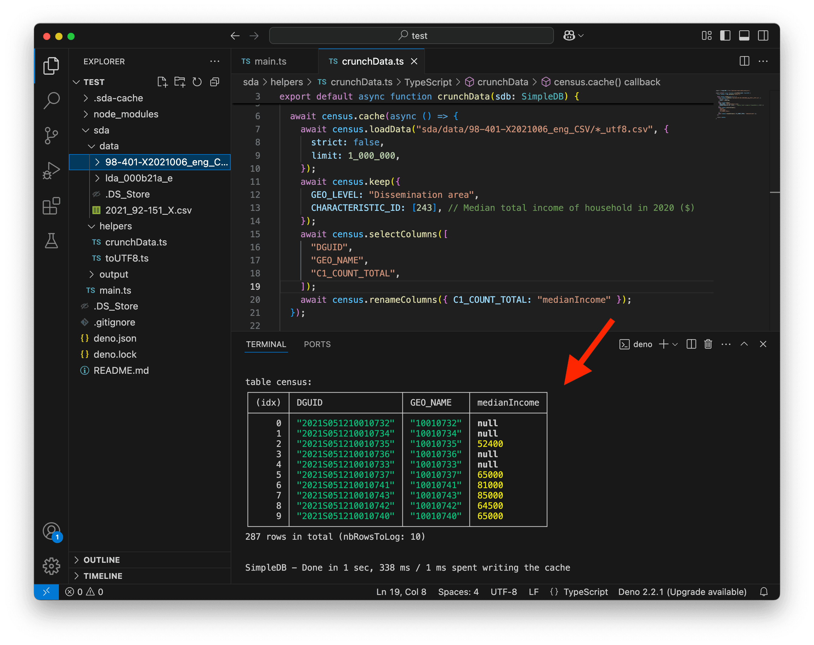
This is looking much better! We can now focus on adding the metropolitan area names.
The metropolitan areas
First try
Let’s try to load the names which are in the 2021_92-151_X.csv file. We can update crunchData.ts. We can keep working in the cache method.
import { SimpleDB } from "@nshiab/simple-data-analysis";

export default async function crunchData(sdb: SimpleDB) {
  const census = sdb.newTable("census");

  await census.cache(async () => {
    await census.loadData("sda/data/98-401-X2021006_eng_CSV/*_utf8.csv", {
      strict: false,
      limit: 1_000_000,
    });
    await census.keep({
      GEO_LEVEL: "Dissemination area",
      CHARACTERISTIC_ID: [243], // Median total income of household in 2020 ($)
    });
    await census.selectColumns([
      "DGUID",
      "GEO_NAME",
      "C1_COUNT_TOTAL",
    ]);
    await census.renameColumns({ C1_COUNT_TOTAL: "medianIncome" });

    const names = sdb.newTable("names");
    await names.loadData("sda/data/2021_92-151_X.csv");
    await names.logTable();
  });

  return census;
}
We know this error! It’s the encoding again!
Re-encoding again
Let’s update toUTF8.ts to convert this CSV file too. We comment out the previous code because we don’t need to reconvert the census files.
import { reencode } from "@nshiab/journalism";

// const regions = [
//   "Atlantic",
//   "BritishColumbia",
//   "Ontario",
//   "Prairies",
//   "Quebec",
//   "Territories",
// ];

// for (const r of regions) {
//   console.log(`Processing ${r}`);

//   const newFile =
//     `sda/data/98-401-X2021006_eng_CSV/98-401-X2021006_English_CSV_data_${r}_utf8.csv`;
//   const originalFile =
//     `sda/data/98-401-X2021006_eng_CSV/98-401-X2021006_English_CSV_data_${r}.csv`;

//   await reencode(originalFile, newFile, "windows-1252", "utf-8");

//   console.log(`Done with ${r}`);
// }

console.log(`Processing names data`);
await reencode(
  "sda/data/2021_92-151_X.csv",
  "sda/data/2021_92-151_X_utf8.csv",
  "windows-1252",
  "utf-8",
);
console.log("Done with names data");
Stop watching main.ts in your terminal (CTRL + C) and run deno task toUTF8.
Now, let’s load our new file sda/data/2021_92-151_X_utf8.csv in crunchData.ts.
import { SimpleDB } from "@nshiab/simple-data-analysis";

export default async function crunchData(sdb: SimpleDB) {
  const census = sdb.newTable("census");

  await census.cache(async () => {
    await census.loadData("sda/data/98-401-X2021006_eng_CSV/*_utf8.csv", {
      strict: false,
      limit: 1_000_000,
    });
    await census.keep({
      GEO_LEVEL: "Dissemination area",
      CHARACTERISTIC_ID: [243], // Median total income of household in 2020 ($)
    });
    await census.selectColumns([
      "DGUID",
      "GEO_NAME",
      "C1_COUNT_TOTAL",
    ]);
    await census.renameColumns({ C1_COUNT_TOTAL: "medianIncome" });

    const names = sdb.newTable("names");
    await names.loadData("sda/data/2021_92-151_X_utf8.csv");
    await names.logTable();
  });

  return census;
}
Another error… Again, we have to set the strict option to false.
import { SimpleDB } from "@nshiab/simple-data-analysis";

export default async function crunchData(sdb: SimpleDB) {
  const census = sdb.newTable("census");

  await census.cache(async () => {
    await census.loadData("sda/data/98-401-X2021006_eng_CSV/*_utf8.csv", {
      strict: false,
      limit: 1_000_000,
    });
    await census.keep({
      GEO_LEVEL: "Dissemination area",
      CHARACTERISTIC_ID: [243], // Median total income of household in 2020 ($)
    });
    await census.selectColumns([
      "DGUID",
      "GEO_NAME",
      "C1_COUNT_TOTAL",
    ]);
    await census.renameColumns({ C1_COUNT_TOTAL: "medianIncome" });

    const names = sdb.newTable("names");
    await names.loadData("sda/data/2021_92-151_X_utf8.csv", { strict: false });
    await names.logTable();
  });

  return census;
}
And now it works! But this file has a whopping 63 columns. 😳
Filtering
If you read the documentation (and know your Census pretty well 🥸), you’ll realize that you only need two columns, after filtering CMATYPE_RMRGENRE for the B type to keep only metropolitan areas.
Because the file contains data for different geographical levels, we remove duplicates created by selecting just two columns. And since the goal is to add the metropolitan names to our census table, we rename the column DADGUID_ADIDUGD to DGUID to easily join the two tables. We also rename CMANAME_RMRNOM to CMA for convenience.
Here’s an updated version of crunchData.ts.
import { SimpleDB } from "@nshiab/simple-data-analysis";

export default async function crunchData(sdb: SimpleDB) {
  const census = sdb.newTable("census");

  await census.cache(async () => {
    await census.loadData("sda/data/98-401-X2021006_eng_CSV/*_utf8.csv", {
      strict: false,
      limit: 1_000_000,
    });
    await census.keep({
      GEO_LEVEL: "Dissemination area",
      CHARACTERISTIC_ID: [243], // Median total income of household in 2020 ($)
    });
    await census.selectColumns([
      "DGUID",
      "GEO_NAME",
      "C1_COUNT_TOTAL",
    ]);
    await census.renameColumns({ C1_COUNT_TOTAL: "medianIncome" });

    const names = sdb.newTable("names");
    await names.loadData("sda/data/2021_92-151_X_utf8.csv", { strict: false });
    await names.keep({
      CMATYPE_RMRGENRE: "B",
    });
    await names.selectColumns(["DADGUID_ADIDUGD", "CMANAME_RMRNOM"]);
    await names.removeDuplicates();
    await names.renameColumns({
      DADGUID_ADIDUGD: "DGUID",
      CMANAME_RMRNOM: "CMA",
    });
    await census.join(names);
  });

  return census;
}
Victory! We now have the metropolitan area name for each dissemination area! 🥳
The dissemination areas boundaries
Simplifying
Since we want to make a map, we need the dissemination areas boundaries. We downloaded them earlier as the zipped file lda_000b21a_e.zip (and I told you not to unzip them 😬).
Statistics Canada provides very detailed geospatial data. But since we only want to draw maps, we don’t need a very high level of detail. A simplified version would be enough and would make our code run faster.
One of my favorite tools to simplify geospatial data is mapshaper.org. Go give them a ⭐ on GitHub if you have an account!
Go on the website and drag-and-drop lda_000b21a_e.zip on the page. Note that you can’t drag-and-drop from VS Code. Do it from your folder using your computer’s Finder or File Explorer.
After a few seconds, you’ll see all the dissemination areas.

You can now click on Simplify on the top right corner and select the following options:
prevent shape removalVisvalingam / weighted area
Click on Apply!

For the next step, I usually zoom in on a high-density area, like Montreal. Then, using the top slider, I aim for a simplification threshold that doesn’t alter the overall shapes.
Here, 10% works pretty well. Note that you can type in the percentage that you want directly too.

And the next step is to export the simplified data!
Click on the Export button in the top right corner, keep the file format as the original Shapefile, and hit Export.

You can now rename this file lda_000b21a_e_simplified.shp.zip (notice I added .shp.zip for the file extension to help SDA understand it’s a shapefile) and move it to your data folder.
Instead of 197 MB, our geospatial data now weighs just 27 MB, which will help speed up our computations and map drawing!
Loading the geometries
To load the geometries, we can use the loadGeoData method. Don’t forget to modify the file extension of your simplified Shapefile to .shp.zip. The shp is important for SDA. Without it, SDA doesn’t recognize the file as a Shapefile and can’t load it correctly.
When you load new geospatial data, it’s always important to check the projection. Below, we use the logProjections method for that.
import { SimpleDB } from "@nshiab/simple-data-analysis";

export default async function crunchData(sdb: SimpleDB) {
  const census = sdb.newTable("census");

  await census.cache(async () => {
    await census.loadData("sda/data/98-401-X2021006_eng_CSV/*_utf8.csv", {
      strict: false,
      limit: 1_000_000,
    });
    await census.keep({
      GEO_LEVEL: "Dissemination area",
      CHARACTERISTIC_ID: [243], // Median total income of household in 2020 ($)
    });
    await census.selectColumns([
      "DGUID",
      "GEO_NAME",
      "C1_COUNT_TOTAL",
    ]);
    await census.renameColumns({ C1_COUNT_TOTAL: "medianIncome" });

    const names = sdb.newTable("names");
    await names.loadData("sda/data/2021_92-151_X_utf8.csv", { strict: false });
    await names.keep({
      CMATYPE_RMRGENRE: "B",
    });
    await names.selectColumns(["DADGUID_ADIDUGD", "CMANAME_RMRNOM"]);
    await names.removeDuplicates();
    await names.renameColumns({
      DADGUID_ADIDUGD: "DGUID",
      CMANAME_RMRNOM: "CMA",
    });
    await census.join(names);

    const disseminationAreas = sdb.newTable("disseminationAreas");
    await disseminationAreas.loadGeoData(
      "sda/data/lda_000b21a_e_simplified.shp.zip",
    );
    await disseminationAreas.logProjections()
    await disseminationAreas.logTable();
  });

  return census;
}
We have no problem loading the geospatial data. We can see the 57,932 dissemination areas as rows with their properties and geometries.
But the projection proj=lcc with its units=m is problematic. Statistics Canada uses the Lambert conic conformal projection with coordinates in meters. For many SDA methods to work properly, we need the coordinates with the WGS84 projection using latitude and longitude.
But don’t worry, SDA has you covered. You just need to pass the option { toWGS84: true } to convert your geospatial data to the right format.
While at it, let’s select only the columns we are interested in:
DGUID, which is the unique ID for dissemination areas. We will use it to join the geometries to the census data.geom, which stores the geometries.
And let’s join the disseminationAreas table to the census table! Since we have a DGUID in each table, SDA will use it to match the dissemination areas’ census data with the right boundaries.
import { SimpleDB } from "@nshiab/simple-data-analysis";

export default async function crunchData(sdb: SimpleDB) {
  const census = sdb.newTable("census");

  await census.cache(async () => {
    await census.loadData("sda/data/98-401-X2021006_eng_CSV/*_utf8.csv", {
      strict: false,
      limit: 1_000_000,
    });
    await census.keep({
      GEO_LEVEL: "Dissemination area",
      CHARACTERISTIC_ID: [243], // Median total income of household in 2020 ($)
    });
    await census.selectColumns([
      "DGUID",
      "GEO_NAME",
      "C1_COUNT_TOTAL",
    ]);
    await census.renameColumns({ C1_COUNT_TOTAL: "medianIncome" });

    const names = sdb.newTable("names");
    await names.loadData("sda/data/2021_92-151_X_utf8.csv", { strict: false });
    await names.keep({
      CMATYPE_RMRGENRE: "B",
    });
    await names.selectColumns(["DADGUID_ADIDUGD", "CMANAME_RMRNOM"]);
    await names.removeDuplicates();
    await names.renameColumns({
      DADGUID_ADIDUGD: "DGUID",
      CMANAME_RMRNOM: "CMA",
    });
    await census.join(names);

    const disseminationAreas = sdb.newTable("disseminationAreas");
    await disseminationAreas.loadGeoData(
      "sda/data/lda_000b21a_e_simplified.shp.zip",
      { toWGS84: true },
    );
    await disseminationAreas.selectColumns(["DGUID", "geom"]);
    await census.join(disseminationAreas);
  });

  return census;
}
Our data is finally complete! We have our dissemination areas with their median total household income, the name of their metropolitan area, and their boundaries!
We can remove the limit option on line 9 and select just the three columns that we will use going forward. We can also remove rows with missing values.
Let’s run everything now!
import { SimpleDB } from "@nshiab/simple-data-analysis";

export default async function crunchData(sdb: SimpleDB) {
  const census = sdb.newTable("census");

  await census.cache(async () => {
    await census.loadData("sda/data/98-401-X2021006_eng_CSV/*_utf8.csv", {
      strict: false,
    });
    await census.keep({
      GEO_LEVEL: "Dissemination area",
      CHARACTERISTIC_ID: [243], // Median total income of household in 2020 ($)
    });
    await census.selectColumns([
      "DGUID",
      "GEO_NAME",
      "C1_COUNT_TOTAL",
    ]);
    await census.renameColumns({ C1_COUNT_TOTAL: "medianIncome" });

    const names = sdb.newTable("names");
    await names.loadData("sda/data/2021_92-151_X_utf8.csv", { strict: false });
    await names.keep({
      CMATYPE_RMRGENRE: "B",
    });
    await names.selectColumns(["DADGUID_ADIDUGD", "CMANAME_RMRNOM"]);
    await names.removeDuplicates();
    await names.renameColumns({
      DADGUID_ADIDUGD: "DGUID",
      CMANAME_RMRNOM: "CMA",
    });
    await census.join(names);

    const disseminationAreas = sdb.newTable("disseminationAreas");
    await disseminationAreas.loadGeoData(
      "sda/data/lda_000b21a_e_simplified.shp.zip",
      { toWGS84: true },
    );
    await disseminationAreas.selectColumns(["DGUID", "geom"]);
    await census.join(disseminationAreas);
    await census.selectColumns(["medianIncome", "CMA", "geom"]);
    await census.removeMissing();
  });

  return census;
}
We now have our data for around 37 thousand dissemination areas located in metropolitan areas.
And since all of this code is within the cache method, it will run just once and let us work quickly on the next steps! As shown above, on the first pass, the code took 1 min 31 seconds to run on my computer. But on the second, it took only 97 ms. 😏

Structuring, formatting, filtering, and cleaning the data is often the longest step in data analysis and visualization. 🫠 But it’s also extremely important to do it properly to avoid errors in your analysis and visualizations.
Always take the time to read the data documentation. It might feel like a waste of time at the beginning, but it will actually save you a lot of time down the road. I’ve been there. Trust me. 🫣
Answering the question
Variation from the median
The question we want to answer is:
- For each Canadian metropolitan area, which dissemination areas have household incomes above or below the median?
So we need to find the median household total income for each metropolitan area. This is easy to do with the method summarize.
Note that we can work outside the cache method now. With the data cleaned up and filtered, this is an easy lift.
import { SimpleDB } from "@nshiab/simple-data-analysis";

export default async function crunchData(sdb: SimpleDB) {
  const census = sdb.newTable("census");

  await census.cache(async () => {
    await census.loadData("sda/data/98-401-X2021006_eng_CSV/*_utf8.csv", {
      strict: false,
    });
    await census.keep({
      GEO_LEVEL: "Dissemination area",
      CHARACTERISTIC_ID: [243], // Median total income of household in 2020 ($)
    });
    await census.selectColumns([
      "DGUID",
      "GEO_NAME",
      "C1_COUNT_TOTAL",
    ]);
    await census.renameColumns({ C1_COUNT_TOTAL: "medianIncome" });

    const names = sdb.newTable("names");
    await names.loadData("sda/data/2021_92-151_X_utf8.csv", { strict: false });
    await names.keep({
      CMATYPE_RMRGENRE: "B",
    });
    await names.selectColumns(["DADGUID_ADIDUGD", "CMANAME_RMRNOM"]);
    await names.removeDuplicates();
    await names.renameColumns({
      DADGUID_ADIDUGD: "DGUID",
      CMANAME_RMRNOM: "CMA",
    });
    await census.join(names);

    const disseminationAreas = sdb.newTable("disseminationAreas");
    await disseminationAreas.loadGeoData(
      "sda/data/lda_000b21a_e_simplified.shp.zip",
      { toWGS84: true },
    );
    await disseminationAreas.selectColumns(["DGUID", "geom"]);
    await census.join(disseminationAreas);
    await census.selectColumns(["medianIncome", "CMA", "geom"]);
    await census.removeMissing();
  });

  const medians = await census.summarize({
    values: "medianIncome",
    categories: "CMA",
    summaries: "median",
    outputTable: "medians",
  });
  await medians.logTable();

  return census;
}
Now that we have the median for each CMA in the medians table, we can join the medians table to the census table. Since both have the CMA column, SDA will be able to easily match the rows. For convenience, we can remove the value column from medians before doing the join.
We can now add a new column varPerc with the percentage variation from the median for each dissemination area. We can round the values too. This is what we will use to color our maps.
import { SimpleDB } from "@nshiab/simple-data-analysis";

export default async function crunchData(sdb: SimpleDB) {
  const census = sdb.newTable("census");

  await census.cache(async () => {
    await census.loadData("sda/data/98-401-X2021006_eng_CSV/*_utf8.csv", {
      strict: false,
    });
    await census.keep({
      GEO_LEVEL: "Dissemination area",
      CHARACTERISTIC_ID: [243], // Median total income of household in 2020 ($)
    });
    await census.selectColumns([
      "DGUID",
      "GEO_NAME",
      "C1_COUNT_TOTAL",
    ]);
    await census.renameColumns({ C1_COUNT_TOTAL: "medianIncome" });

    const names = sdb.newTable("names");
    await names.loadData("sda/data/2021_92-151_X_utf8.csv", { strict: false });
    await names.keep({
      CMATYPE_RMRGENRE: "B",
    });
    await names.selectColumns(["DADGUID_ADIDUGD", "CMANAME_RMRNOM"]);
    await names.removeDuplicates();
    await names.renameColumns({
      DADGUID_ADIDUGD: "DGUID",
      CMANAME_RMRNOM: "CMA",
    });
    await census.join(names);

    const disseminationAreas = sdb.newTable("disseminationAreas");
    await disseminationAreas.loadGeoData(
      "sda/data/lda_000b21a_e_simplified.shp.zip",
      { toWGS84: true },
    );
    await disseminationAreas.selectColumns(["DGUID", "geom"]);
    await census.join(disseminationAreas);
    await census.selectColumns(["medianIncome", "CMA", "geom"]);
    await census.removeMissing();
  });

  const medians = await census.summarize({
    values: "medianIncome",
    categories: "CMA",
    summaries: "median",
    outputTable: "medians",
  });
  await medians.removeColumns("value");

  await census.join(medians);
  await census.addColumn(
    "varPerc",
    "number",
    `(medianIncome - median) / median * 100`,
  );
  await census.round("varPerc");

  return census;
}
We now have the answer to our question: the variation from the median in each dissemination area for all metropolitan areas.
Time to visualize this!
Making maps
To keep our code organized and to stay mentally sane, let’s create a new file visualizeData.ts in helpers.
The new function will need the census table and will just log it for now.
import { SimpleTable } from "@nshiab/simple-data-analysis";

export default async function visualizeData(census: SimpleTable) {
  await census.logTable();
}
And let’s update main.ts to call this new function.
import { SimpleDB } from "@nshiab/simple-data-analysis";
import crunchData from "./helpers/crunchData.ts";
import visualizeData from "./helpers/visualizeData.ts";

const sdb = new SimpleDB({ cacheVerbose: true });

const census = await crunchData(sdb);
await visualizeData(census);

await sdb.done();
We want to draw a map for each metropolitan area, so first, let’s retrieve all unique metropolitan areas in our data.
Then, we can loop over them, clone the census table, and keep only the rows with the right CMA.
As you can see in the screenshot below the new code, when you don’t specify a name for tables, SDA automatically names them table0, table1, etc. Here, we can see that the last table is table42, meaning we are looping over 43 metropolitan areas.
To know the number of metropolitan areas, you could also check the .length of allCMAs, since getUniques returns all unique values in a column as an array.
import { SimpleTable } from "@nshiab/simple-data-analysis";

export default async function visualizeData(census: SimpleTable) {
  const allCMAs = await census.getUniques("CMA");

  for (const CMA of allCMAs) {
    const tableCMA = await census.cloneTable();
    await tableCMA.keep({ CMA });
    await tableCMA.logTable();
  }
}
Because the census table has a column CMA and the loop is using the CMA variable too, we can write { CMA } as a shortcut for { CMA: CMA }.
We can now create a function to draw our maps. When we set up everything with setup-sda, we automatically installed Plot. This very powerful data visualization library works very well with SDA and this is what we are going to use to draw our map.
Since it’s the same function to draw all of the maps, we can create it outside of the loop. This function will expect the data as a GeoJSON, with an array of features with properties. To start, let’s draw the dissemination area polygons with the geo mark and let’s color the fill and stroke with the values we computed in the varPerc column.
In the loop, we can pass this function to the method writeMap, which will pass the data from the table as GeoJSON data to our drawing function. We also need to specify where we want the map to be saved, and we use the metropolitan area name to create unique files in the output folder.
Since we are still in our exploration phase to make the maps, let’s break the loop to work just on the first metropolitan area for now. This will allow us to iterate faster and improve our data visualization.
import { SimpleTable } from "@nshiab/simple-data-analysis";
import { geo, plot } from "@observablehq/plot";

export default async function visualizeData(census: SimpleTable) {
  const allCMAs = await census.getUniques("CMA");

  function drawMap(
    data: { features: { properties: { [key: string]: unknown } }[] },
  ) {
    return plot({
      marks: [
        geo(data, { fill: "varPerc", stroke: "varPearc" }),
      ],
    });
  }

  for (const CMA of allCMAs) {
    const tableCMA = await census.cloneTable();
    await tableCMA.keep({ CMA });
    await tableCMA.writeMap(drawMap, `./sda/output/${CMA}.png`);
    break;
  }
}
It’s ugly, but it works!
We can now add a title, subtitle, and caption. We can also use a diverging scale for the colors and restrict the domain to -100% to +100%. We can also tweak the projection. If you want to know more about these customizations, check the Visualizing data lesson.
One thing you might be wondering is why we have data.features[0].properties.CMA for the title.
When this function is run, it won’t know about the CMA variable. So we need to grab the metropolitan name from the data directly. Since we are using writeMap, SDA passes the data as a GeoJSON to this function. In GeoJSON features, the data is stored in the properties object. So we retrieve the name of the metropolitan area by grabbing the first feature and finding the CMA name in its properties.
import { SimpleTable } from "@nshiab/simple-data-analysis";
import { geo, plot } from "@observablehq/plot";

export default async function visualizeData(census: SimpleTable) {
  const allCMAs = await census.getUniques("CMA");

  function drawMap(
    data: { features: { properties: { [key: string]: unknown } }[] },
  ) {
    return plot({
      title: data.features[0].properties.CMA,
      subtitle:
        "Variation from the median household total income at the dissemination area level.",
      caption: "2021 Census, Statistics Canada",
      inset: 10,
      projection: {
        type: "mercator",
        domain: data,
      },
      color: {
        legend: true,
        type: "diverging",
        domain: [-100, 100],
        label: null,
        tickFormat: (d) => {
          if (d > 0) {
            return `+${d}%`;
          } else {
            return `${d}%`;
          }
        },
      },
      marks: [
        geo(data, { fill: "varPerc", stroke: "varPerc" }),
      ],
    });
  }

  for (const CMA of allCMAs) {
    const tableCMA = await census.cloneTable();
    await tableCMA.keep({ CMA });
    await tableCMA.writeMap(drawMap, `./sda/output/${CMA}.png`);
    break;
  }
}
This is looking much better.
One last thing that I like to do in my maps is to add an outline.
Inside the loop, we can clone the tableCMA and merge all the dissemination areas geometries by running the aggregateGeo method. Since this can be quite computationally expensive when there are a lot of dissemination areas, we cache the result.
We can then insert this newly created geometry into the tableCMA.
In the drawMap function, we can add a new geo mark to draw the outline. But we need to filter on the varPerc to make sure that we only draw the outline and not all the dissemination areas again.
import { SimpleTable } from "@nshiab/simple-data-analysis";
import { geo, plot } from "@observablehq/plot";

export default async function visualizeData(census: SimpleTable) {
  const allCMAs = await census.getUniques("CMA");

  function drawMap(
    data: { features: { properties: { [key: string]: unknown } }[] },
  ) {
    return plot({
      title: data.features[0].properties.CMA,
      subtitle:
        "Variation from the median household total income at the dissemination area level.",
      caption: "2021 Census, Statistics Canada",
      inset: 10,
      projection: {
        type: "mercator",
        domain: data,
      },
      color: {
        legend: true,
        type: "diverging",
        domain: [-100, 100],
        label: null,
        tickFormat: (d) => {
          if (d > 0) {
            return `+${d}%`;
          } else {
            return `${d}%`;
          }
        },
      },
      marks: [
        geo(
          data.features.filter((d) => typeof d.properties.varPerc === "number"),
          { fill: "varPerc", stroke: "varPerc" },
        ),
        geo(data.features.filter((d) => d.properties.varPerc === null), {
          stroke: "black",
          opacity: 0.5,
        }),
      ],
    });
  }

  for (const CMA of allCMAs) {
    const tableCMA = await census.cloneTable();
    await tableCMA.keep({ CMA });

    const outline = await tableCMA.cloneTable();
    await outline.cache(async () => {
      await outline.aggregateGeo("union");
    });
    await tableCMA.insertTables(outline);

    await tableCMA.writeMap(drawMap, `./sda/output/${CMA}.png`);
    break;
  }
}
The difference is subtle, but it’s important to see the holes in the metropolitan area geometry.
Now that we are happy with our map’s look, it’s time to remove the break statement on line 57! Let’s create 43 maps! Run everything!
If you inspect the maps after running your code, you’ll notice a few problems.

First, you can see that some folders have been created for some metropolitan areas in the output folder. It’s because some names have / in them! We need to replace this character with something else before passing it to writeMap.
We can update visualizeData.ts to fix that.
import { SimpleTable } from "@nshiab/simple-data-analysis";
import { geo, plot } from "@observablehq/plot";

export default async function visualizeData(census: SimpleTable) {
  const allCMAs = await census.getUniques("CMA");

  function drawMap(
    data: { features: { properties: { [key: string]: unknown } }[] },
  ) {
    return plot({
      title: data.features[0].properties.CMA,
      subtitle:
        "Variation from the median household total income at the dissemination area level.",
      caption: "2021 Census, Statistics Canada",
      inset: 10,
      projection: {
        type: "mercator",
        domain: data,
      },
      color: {
        legend: true,
        type: "diverging",
        domain: [-100, 100],
        label: null,
        tickFormat: (d) => {
          if (d > 0) {
            return `+${d}%`;
          } else {
            return `${d}%`;
          }
        },
      },
      marks: [
        geo(
          data.features.filter((d) => typeof d.properties.varPerc === "number"),
          { fill: "varPerc", stroke: "varPerc" },
        ),
        geo(data.features.filter((d) => d.properties.varPerc === null), {
          stroke: "black",
          opacity: 0.5,
        }),
      ],
    });
  }

  for (const CMA of allCMAs) {
    const tableCMA = await census.cloneTable();
    await tableCMA.keep({ CMA });

    const outline = await tableCMA.cloneTable();
    await outline.cache(async () => {
      await outline.aggregateGeo("union");
    });
    await tableCMA.insertTables(outline);

    await tableCMA.writeMap(
      drawMap,
      `./sda/output/${(CMA as string).replaceAll("/", "-")}.png`,
    );
  }
}
We can also see that the outline for some cities is not right and the map for Montréal is just one gigantic polygon. This usually happens when some geometries are invalid. Simplification often creates invalid geometries. Luckily, we can call the fixGeo method to the rescue!
We can update crunchData.ts, within the cache method, to fix the geometries after loading the geospatial data.
import { SimpleDB } from "@nshiab/simple-data-analysis";

export default async function crunchData(sdb: SimpleDB) {
  const census = sdb.newTable("census");

  await census.cache(async () => {
    await census.loadData("sda/data/98-401-X2021006_eng_CSV/*_utf8.csv", {
      strict: false,
    });
    await census.keep({
      GEO_LEVEL: "Dissemination area",
      CHARACTERISTIC_ID: [243], // Median total income of household in 2020 ($)
    });
    await census.selectColumns([
      "DGUID",
      "GEO_NAME",
      "C1_COUNT_TOTAL",
    ]);
    await census.renameColumns({ C1_COUNT_TOTAL: "medianIncome" });

    const names = sdb.newTable("names");
    await names.loadData("sda/data/2021_92-151_X_utf8.csv", { strict: false });
    await names.keep({
      CMATYPE_RMRGENRE: "B",
    });
    await names.selectColumns(["DADGUID_ADIDUGD", "CMANAME_RMRNOM"]);
    await names.removeDuplicates();
    await names.renameColumns({
      DADGUID_ADIDUGD: "DGUID",
      CMANAME_RMRNOM: "CMA",
    });
    await census.join(names);

    const disseminationAreas = sdb.newTable("disseminationAreas");
    await disseminationAreas.loadGeoData(
      "sda/data/lda_000b21a_e_simplified.shp.zip",
      { toWGS84: true },
    );
    await disseminationAreas.fixGeo();
    await disseminationAreas.selectColumns(["DGUID", "geom"]);
    await census.join(disseminationAreas);
    await census.selectColumns(["medianIncome", "CMA", "geom"]);
    await census.removeMissing();
  });

  const medians = await census.summarize({
    values: "medianIncome",
    categories: "CMA",
    summaries: "median",
    outputTable: "medians",
  });
  await medians.removeColumns("value");

  await census.join(medians);
  await census.addColumn(
    "varPerc",
    "number",
    `(medianIncome - median) / median * 100`,
  );
  await census.round("varPerc");

  return census;
}
Now, stop watching main.ts (CTRL + C in your terminal) and delete .temp and .sda-cache manually or by running deno task clean. Remove everything in the output folder as well.
And let’s rerun everything from scratch!

Amazing! It runs smoothly and all of our problems disappeared. 😁
On my computer, our code was able to crunch all of the data and draw all of the maps in 2 minutes 46 seconds. But thanks to our clever caching, if I need to tweak the look of the maps, it takes just 32 seconds to rewrite all of the 43 maps.
By the way, here, we are saving our maps as images, but if you want vectors to edit them in Illustrator or other design tools, just replace .png with .svg in writeMap.
Conclusion
What a journey! Crunching big datasets with multiple tables storing tabular and geospatial data is not an easy task.
But I hope this real-life example showed you how you can cut through GB of data like it was butter with SDA. 🧈
Have fun with your next data project and feel free to reach out if you want to share what you are making with SDA or if you have any questions! 😊